Example : multiclass classification of the Iris dataset

This example script can be found at aweSOM/examples/iris/iris.ipynb

Single aweSOM realization

Import aweSOM and iris dataset

from aweSOM import Lattice
import numpy as np
import matplotlib.pyplot as plt
from sklearn.datasets import load_iris

Basic information about the dataset

iris = load_iris()

print("Shape of the data :", iris.data.shape)
print("Labeled classes :", iris.target_names)
print("Features in the set :", iris.feature_names)

Shape of the data : (150, 4)
Labeled classes : ['setosa' 'versicolor' 'virginica']
Features in the set : ['sepal length (cm)', 'sepal width (cm)', 'petal length (cm)', 'petal width (cm)']

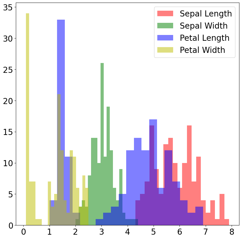
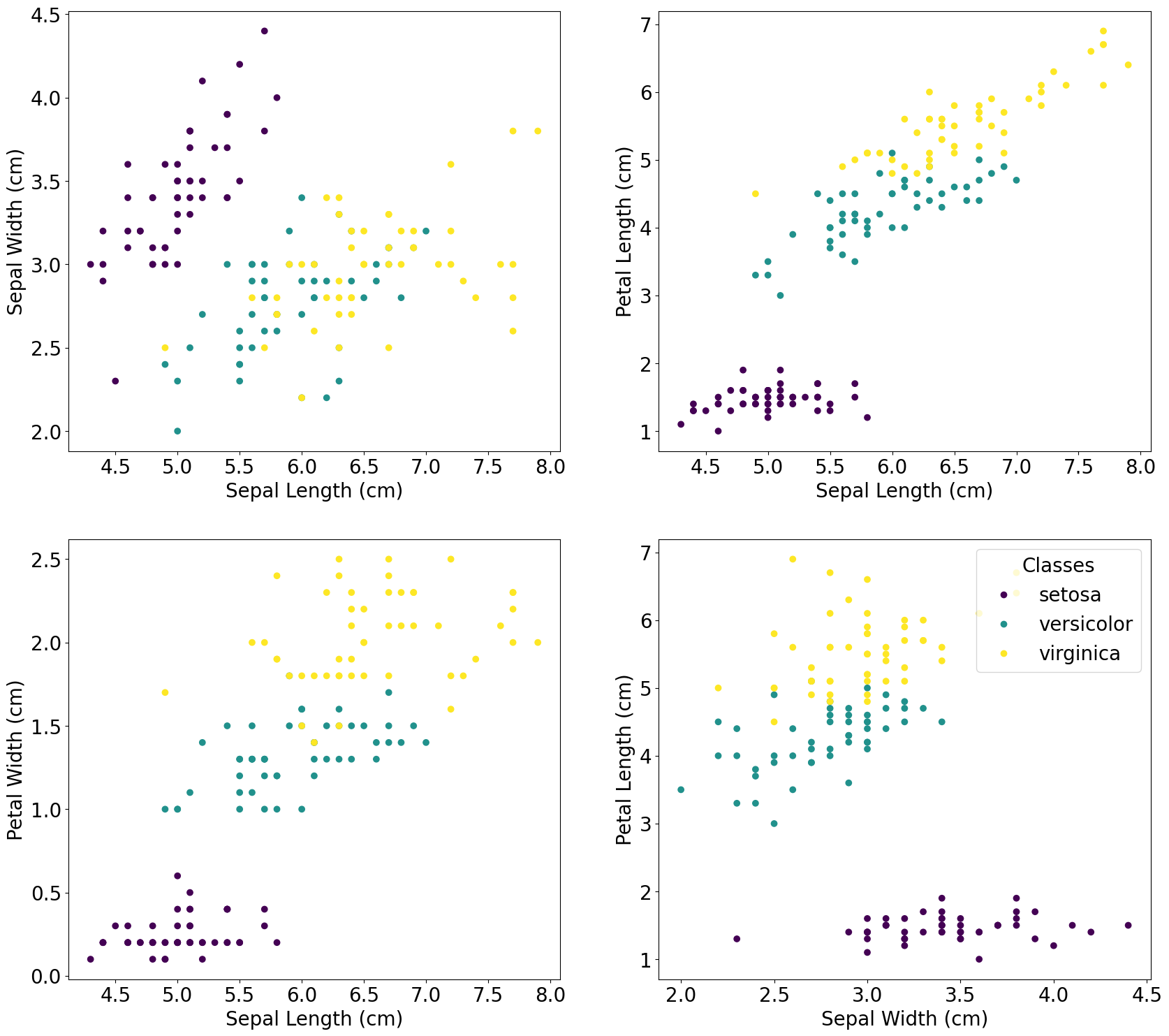
Visualize the dataset in a few different ways

plt.rcParams.update({'font.size': 20})

# Histogram
plt.figure(figsize=(10, 10))
plt.hist(iris.data[:,0], bins=20, color='r', alpha=0.5, label='Sepal Length')
plt.hist(iris.data[:,1], bins=20, color='g', alpha=0.5, label='Sepal Width')
plt.hist(iris.data[:,2], bins=20, color='b', alpha=0.5, label='Petal Length')
plt.hist(iris.data[:,3], bins=20, color='y', alpha=0.5, label='Petal Width')
plt.legend()
plt.show()

# Scatter plots
fig, axs = plt.subplots(2, 2, figsize=(20, 18))
scatter = axs[0,0].scatter(iris.data[:,0], iris.data[:,1], c=iris.target, cmap='viridis')
axs[0,0].set_xlabel('Sepal Length (cm)')
axs[0,0].set_ylabel('Sepal Width (cm)')
axs[0,1].scatter(iris.data[:,0], iris.data[:,2], c=iris.target, cmap='viridis')
axs[0,1].set_xlabel('Sepal Length (cm)')
axs[0,1].set_ylabel('Petal Length (cm)')
axs[1,0].scatter(iris.data[:,0], iris.data[:,3], c=iris.target, cmap='viridis')
axs[1,0].set_xlabel('Sepal Length (cm)')
axs[1,0].set_ylabel('Petal Width (cm)')
axs[1,1].scatter(iris.data[:,1], iris.data[:,2], c=iris.target, cmap='viridis')
axs[1,1].set_xlabel('Sepal Width (cm)')
axs[1,1].set_ylabel('Petal Length (cm)')
plt.legend(scatter.legend_elements()[0], iris.target_names, loc="upper right", title="Classes")

<matplotlib.legend.Legend at 0x155503021b50>

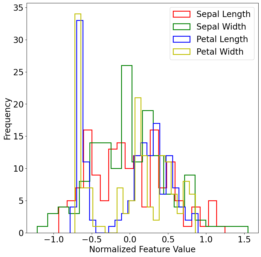
Pre-processing step : normalize data with either MinMaxScaler (shift the distribution to between 0 and 1) or StandardScaler (shift the mean to 0 and standard deviation of the sample to 1). Here we use the custom scaler described in Ha et al. 2024

import aweSOM.run_som as rs
iris_data_transformed = rs.manual_scaling(iris.data)

plt.figure(figsize=(10, 10))
plt.hist(iris_data_transformed[:,0], bins=20, color='r', label='Sepal Length', histtype='step', linewidth=2)
plt.hist(iris_data_transformed[:,1], bins=20, color='g', label='Sepal Width', histtype='step', linewidth=2)
plt.hist(iris_data_transformed[:,2], bins=20, color='b', label='Petal Length', histtype='step', linewidth=2)
plt.hist(iris_data_transformed[:,3], bins=20, color='y', label='Petal Width', histtype='step', linewidth=2)
plt.xlabel('Normalized Feature Value')
plt.ylabel('Frequency')
plt.legend()
plt.show()

Example lattice:

Initialize the SOM map

xdim, ydim = 20, 8 # small map since there are only 150 samples
alpha_0 = 1.
train = 1000000

print(f'constructing aweSOM lattice for xdim={xdim}, ydim={ydim}, alpha={alpha_0}, train={train}...', flush=True)
map=Lattice(xdim, ydim, alpha_0, train, )

constructing aweSOM lattice for xdim=20, ydim=8, alpha=1.0, train=1000000...

Train the SOM with only one batch

labels = iris.target
feature_names = iris.feature_names

map.train_lattice(iris_data_transformed,feature_names,labels,)
lattice = map.lattice

starting epoch is:  0
stopping epoch is:  1000000
Saving lattice every  5000  epochs
Begin training
Evaluating epoch =  0
Decaying learning rate to 0.75 at epoch 40000
Decaying learning rate to 0.5625 at epoch 80000
Evaluating epoch =  100000
Decaying learning rate to 0.421875 at epoch 120000
Decaying learning rate to 0.31640625 at epoch 160000
Evaluating epoch =  200000
Decaying learning rate to 0.2373046875 at epoch 200000
Decaying learning rate to 0.177978515625 at epoch 240000
Decaying learning rate to 0.13348388671875 at epoch 280000
Evaluating epoch =  300000
Decaying learning rate to 0.1001129150390625 at epoch 320000
Decaying learning rate to 0.07508468627929688 at epoch 360000
Evaluating epoch =  400000
Decaying learning rate to 0.056313514709472656 at epoch 400000
Decaying learning rate to 0.04223513603210449 at epoch 440000
Decaying learning rate to 0.03167635202407837 at epoch 480000
Evaluating epoch =  500000
Shrinking neighborhood size to 21 at epoch 519210
Decaying learning rate to 0.023757264018058777 at epoch 520000
Shrinking neighborhood size to 20 at epoch 538440
Shrinking neighborhood size to 19 at epoch 557670
Decaying learning rate to 0.017817948013544083 at epoch 560000
Shrinking neighborhood size to 18 at epoch 576900
Shrinking neighborhood size to 17 at epoch 596130
Evaluating epoch =  600000
Decaying learning rate to 0.013363461010158062 at epoch 600000
Shrinking neighborhood size to 16 at epoch 615360
Shrinking neighborhood size to 15 at epoch 634590
Decaying learning rate to 0.010022595757618546 at epoch 640000
Shrinking neighborhood size to 14 at epoch 653820
Shrinking neighborhood size to 13 at epoch 673050
Decaying learning rate to 0.00751694681821391 at epoch 680000
Shrinking neighborhood size to 12 at epoch 692280
Evaluating epoch =  700000
Shrinking neighborhood size to 11 at epoch 711510
Decaying learning rate to 0.005637710113660432 at epoch 720000
Shrinking neighborhood size to 10 at epoch 730740
Shrinking neighborhood size to 9 at epoch 749970
Decaying learning rate to 0.004228282585245324 at epoch 760000
Shrinking neighborhood size to 8 at epoch 769200
Evaluating epoch =  800000
Decaying learning rate to 0.0031712119389339932 at epoch 800000
Decaying learning rate to 0.002378408954200495 at epoch 840000
Decaying learning rate to 0.0017838067156503712 at epoch 880000
Evaluating epoch =  900000
Decaying learning rate to 0.0013378550367377784 at epoch 920000
Decaying learning rate to 0.0010033912775533338 at epoch 960000
Evaluating epoch =  1000000
Terminating from step limit reached at epoch  1000000
Training complete

Visualize result with Umatrix

map.umat = map.compute_umat(smoothing=None)
unique_centroids = map.get_unique_centroids(map.compute_centroids())

unique_centroids['position_x'] = [x+0.5 for x in unique_centroids['position_x']]
unique_centroids['position_y'] = [y+0.5 for y in unique_centroids['position_y']]

X,Y = np.meshgrid(np.arange(xdim)+0.5, np.arange(ydim)+0.5)

plt.figure(dpi=250)
plt.pcolormesh(np.log10(map.umat.T), cmap='viridis')
plt.scatter(unique_centroids['position_x'],unique_centroids['position_y'], color='red', s=10)
plt.colorbar(fraction=0.02)
plt.contour(X, Y, np.log10(map.umat.T), levels=np.linspace(np.log10(np.min(map.umat)),np.log10(np.max(map.umat)), 20), colors='black', alpha=0.5)
plt.gca().set_aspect("equal")
plt.title(rf'UMatrix for {xdim}x{ydim} SOM')

Text(0.5, 1.0, 'UMatrix for 20x8 SOM')

print('Number of centroids:', len(unique_centroids['position_x']))

Number of centroids: 6

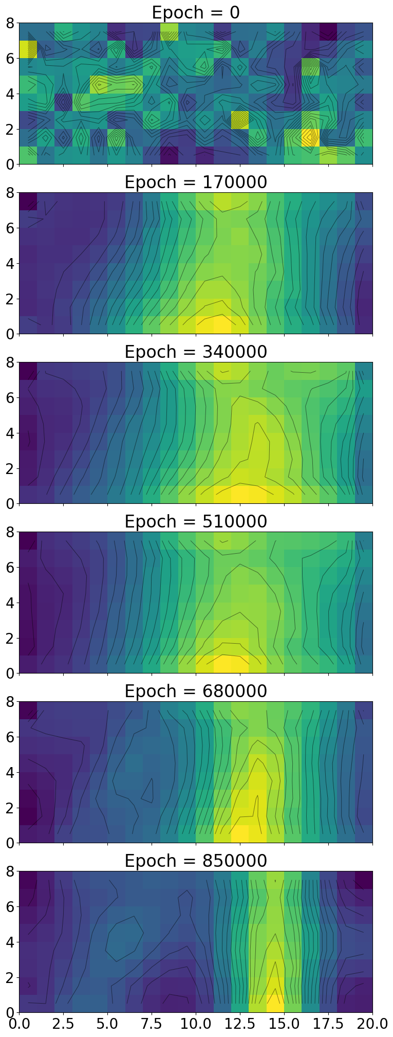
You can also look at the history of the map with umat_history (and lattice_history)

lattice_history = np.array(map.lattice_history)
umat_history = np.array(map.umat_history)
steps = np.linspace(0, lattice_history.shape[0] * map.save_frequency, lattice_history.shape[0], endpoint=False, dtype=int)

xdim = map.xdim
ydim = map.ydim
alpha_0 = map.alpha_0
train = map.train
X,Y = np.meshgrid(np.arange(xdim)+0.5, np.arange(ydim)+0.5)


num_plots = 6
fig, axs = plt.subplots(6, 1, figsize=(10, 25), sharex=True)
fig.subplots_adjust(hspace=0.2)
for i, k in enumerate(range(0, umat_history.shape[0], len(steps)//num_plots+1)):
    umat = umat_history[k]

    axs[i].title.set_text(f'Epoch = {steps[k]}')
    mesh = axs[i].pcolormesh(umat.T, cmap='viridis')
    axs[i].contour(X, Y, umat.T, levels=np.linspace(np.min(umat),np.max(umat), 20), colors='black', alpha=0.5, linewidths=0.7)
    axs[i].set_aspect("equal")

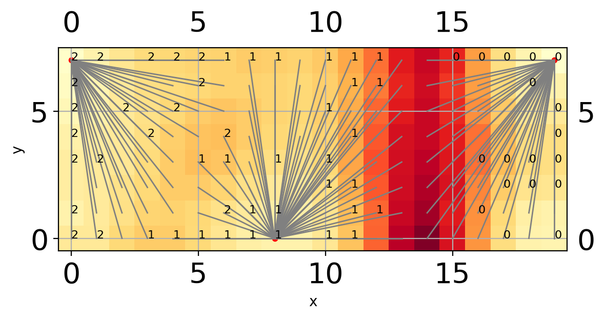
Merge similar centroids

map.umat = map.compute_umat(smoothing=None)
naive_centroids = map.compute_centroids()
merge_threshold = 0.2
merged_centroids = map.merge_similar_centroids(naive_centroids, threshold=merge_threshold)

Centroid A: (np.int64(0), np.int64(1)), count: 11
Centroid B: (np.int64(0), np.int64(7)), count: 35
Merging...
Centroid A: (np.int64(19), np.int64(7)), count: 25
Centroid B: (np.int64(19), np.int64(0)), count: 23
Merging...
Centroid A: (np.int64(9), np.int64(6)), count: 16
Centroid B: (np.int64(8), np.int64(0)), count: 50
Merging...
Number of unique centroids:  3
Minimum cost between centroids:  0.278679788562555

Visualize new centroids after merging

map.plot_heat(map.umat, merge=True, merge_cost=merge_threshold)

Centroid A: (np.int64(0), np.int64(1)), count: 11
Centroid B: (np.int64(0), np.int64(7)), count: 35
Merging...
Centroid A: (np.int64(19), np.int64(7)), count: 25
Centroid B: (np.int64(19), np.int64(0)), count: 23
Merging...
Centroid A: (np.int64(9), np.int64(6)), count: 16
Centroid B: (np.int64(8), np.int64(0)), count: 50
Merging...
Number of unique centroids:  3
Minimum cost between centroids:  0.278679788562555
Unique centroids :  {'position_x': [np.int64(19), np.int64(0), np.int64(8)], 'position_y': [np.int64(7), np.int64(7), np.int64(0)]}
Begin matching points with nodes
i = i =  120
i =  45
i =  90
 0
i =  60
i =  105
i =  15
i =  135
i =  75
i =  30

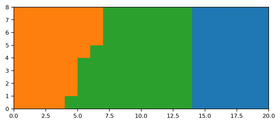
Project data onto lattice

final_clusters = map.assign_cluster_to_lattice(smoothing=None,merge_cost=merge_threshold)

plt.figure(dpi=200)
plt.pcolormesh(final_clusters.T, cmap='tab10', clim=[0,10])
plt.gca().set_aspect("equal")
plt.show()

Centroid A: (np.int64(0), np.int64(1)), count: 11
Centroid B: (np.int64(0), np.int64(7)), count: 35
Merging...
Centroid A: (np.int64(19), np.int64(7)), count: 25
Centroid B: (np.int64(19), np.int64(0)), count: 23
Merging...
Centroid A: (np.int64(9), np.int64(6)), count: 16
Centroid B: (np.int64(8), np.int64(0)), count: 50
Merging...
Number of unique centroids:  3
Minimum cost between centroids:  0.278679788562555
Number of clusters : 3
Centroids:  [(np.int64(19), np.int64(7)), (np.int64(0), np.int64(7)), (np.int64(8), np.int64(0))]

Map cluster ids back to each data point

som_labels = map.assign_cluster_to_data(map.projection_2d, final_clusters)

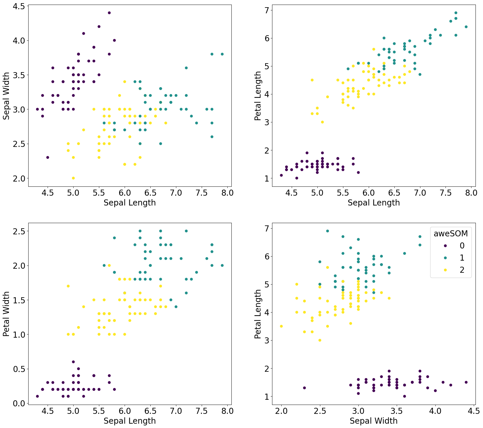
Scatter plot of cluster ids from SOM

plt.rcParams.update({'font.size': 20})
fig, axs = plt.subplots(2, 2, figsize=(20, 18))
scatter = axs[0,0].scatter(iris.data[:,0], iris.data[:,1], c=som_labels, cmap='viridis')
axs[0,0].set_xlabel('Sepal Length')
axs[0,0].set_ylabel('Sepal Width')
axs[0,1].scatter(iris.data[:,0], iris.data[:,2], c=som_labels, cmap='viridis')
axs[0,1].set_xlabel('Sepal Length')
axs[0,1].set_ylabel('Petal Length')
axs[1,0].scatter(iris.data[:,0], iris.data[:,3], c=som_labels, cmap='viridis')
axs[1,0].set_xlabel('Sepal Length')
axs[1,0].set_ylabel('Petal Width')
axs[1,1].scatter(iris.data[:,1], iris.data[:,2], c=som_labels, cmap='viridis')
axs[1,1].set_xlabel('Sepal Width')
axs[1,1].set_ylabel('Petal Length')
axs[1,1].legend(scatter.legend_elements()[0], np.unique(final_clusters), loc="upper right", title="aweSOM")

<matplotlib.legend.Legend at 0x1554fc610ed0>

Visualize a 2d projection between ground truth and aweSOM result

fig, axs = plt.subplots(1, 2, figsize=(20, 10))
scatter_ground = axs[0].scatter(iris.data[:,1], iris.data[:,2], c=iris.target, cmap='viridis')
axs[0].set_xlabel('Sepal Width')
axs[0].set_ylabel('Petal Length')
axs[0].legend(scatter_ground.legend_elements()[0], iris.target_names, loc="upper right", title="Classes")
scatter_som = axs[1].scatter(iris.data[:,1], iris.data[:,2], c=som_labels, cmap='viridis')
axs[1].set_xlabel('Sepal Width')
axs[1].set_ylabel('Petal Length')
axs[1].legend(scatter_som.legend_elements()[0], np.unique(final_clusters), loc="upper right", title="aweSOM")
plt.show()

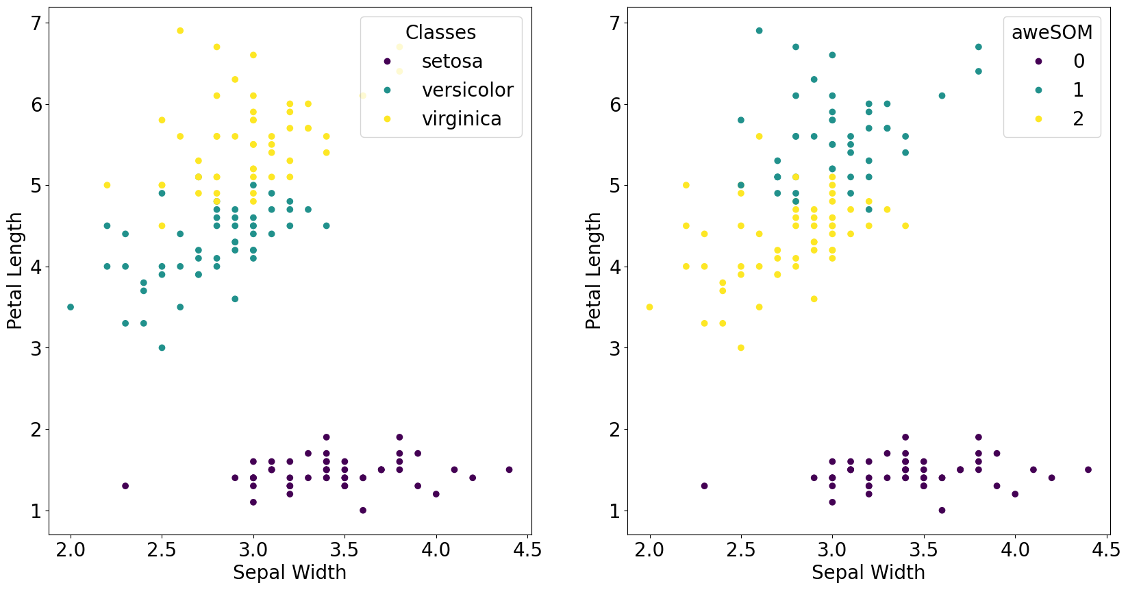
Compare the real label to the inferred label

# Assign cluster number to class label; change manually
label_map = {
    'setosa' : 0,
    'versicolor' : 2,
    'virginica' : 1,
    }
correct_label = 0

for i in range(len(som_labels)):
    if int(som_labels[i]) == label_map[iris.target_names[iris.target[i]]]:
        correct_label += 1

print("Number of correct predictions: ", correct_label)
print("Accuracy = ", correct_label/len(som_labels) * 100, "%")

# Precision and Recall by class
precision = np.zeros(3)
recall = np.zeros(3)

for i in range(3):
    tp = 0
    fp = 0
    fn = 0
    for j in range(len(som_labels)):
        if int(som_labels[j]) == label_map[iris.target_names[i]]:
            if iris.target[j] == i:
                tp += 1
            else:
                fp += 1
        else:
            if iris.target[j] == i:
                fn += 1
    precision[i] = tp/(tp+fp)
    recall[i] = tp/(tp+fn)

print("Precision: ", [float(np.round(precision[i],4))*100 for i in range(3)], "%")
print("Recall: ", [float(np.round(recall[i],4))*100 for i in range(3)], "%")

Number of correct predictions:  139
Accuracy =  92.66666666666666 %
Precision:  [100.0, 85.45, 93.33] %
Recall:  [100.0, 94.0, 84.0] %

Save SOM object (if further examination is warranted)

import pickle
with open('iris_som.pkl', 'wb') as f:
    pickle.dump(map, f)

Stacking multiple aweSOM realizations for SCE analysis

Now we run multiple SOM realizations to obtain SCE clustering

There are files already saved in examples/iris/som_results; run this cell only if you want to generate a different set of aweSOM realizations

from aweSOM.run_som import save_cluster_labels
parameters = {"xdim": [38, 40, 42], "ydim": [14, 16], "alpha_0": [0.1, 0.5], "train": [10000, 50000, 100000]}
merge_threshold = 0.2

for xdim in parameters["xdim"]:
    for ydim in parameters["ydim"]:
        for alpha_0 in parameters["alpha_0"]:
            for train in parameters["train"]:
                print(f'constructing aweSOM lattice for xdim={xdim}, ydim={ydim}, alpha={alpha_0}, train={train}...', flush=True)
                map = Lattice(xdim, ydim, alpha_0, train, )
                map.train_lattice(iris_data_transformed, feature_names, labels)
                # map.umat = map.compute_umat()
                projection_2d = map.map_data_to_lattice()
                final_clusters = map.assign_cluster_to_lattice(smoothing=None, merge_cost=merge_threshold)
                som_labels = map.assign_cluster_to_data(projection_2d, final_clusters)
                save_cluster_labels(som_labels, xdim, ydim, alpha_0, train, name_of_dataset='iris')

The generated realizations (named labels...) are saved in aweSOM/examples/iris/. Move files inside a subfolder, som_results/, before proceeding to next step.

If using pre-generated realizations, the labeled files are already saved in som_results/

import os
original_path = os.getcwd()
os.chdir('som_results/')

Run SCE analysis on the given files, suppress console output

%%capture
%run -i ../../../src/aweSOM/sce.py --subfolder SCE --dims 150

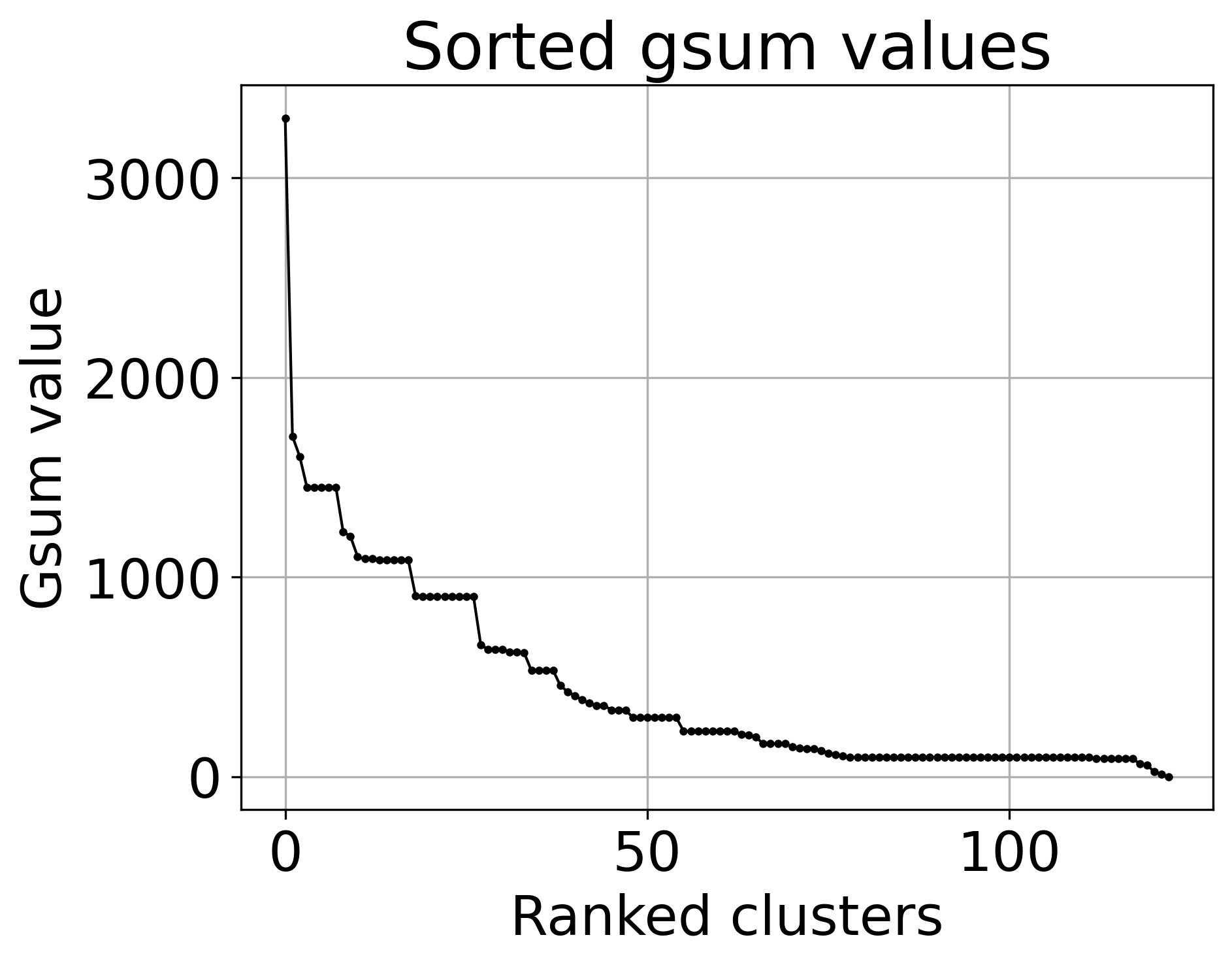
OPTIONAL: To obtain complex SCE clustering via analysis of the breaks in \(G_{\rm sum}\) values, do:

%%capture
os.chdir('SCE/')
%run -i ../../../../src/aweSOM/make_sce_clusters.py --threshold -0.01 --dims 150 --return_gsum

Which then saves two files: gsum_values.png, the ranked \(G_{\rm sum}\) plot, and gsum_deriv.png, the derivative of the previous, which highlights where the large jumps in \(G_{\rm sum}\) are. Each blue X in the map represents the boundary between two SCE clusters.

An optional argument, --save_combined_map, can be added to combine clusters with similar \(G_{\rm sum}\) values together into a set of SCE clusters and save the combined signal strength to a .npy file.

Visualize \(G_{\rm sum}\)

file_path = original_path+'/som_results/SCE/'
file_name = 'multimap_mappings.txt'

from aweSOM.make_sce_clusters import get_gsum_values, plot_gsum_values

ranked_gsum_list, map_list = get_gsum_values(file_path+file_name)

plot_gsum_values(ranked_gsum_list)

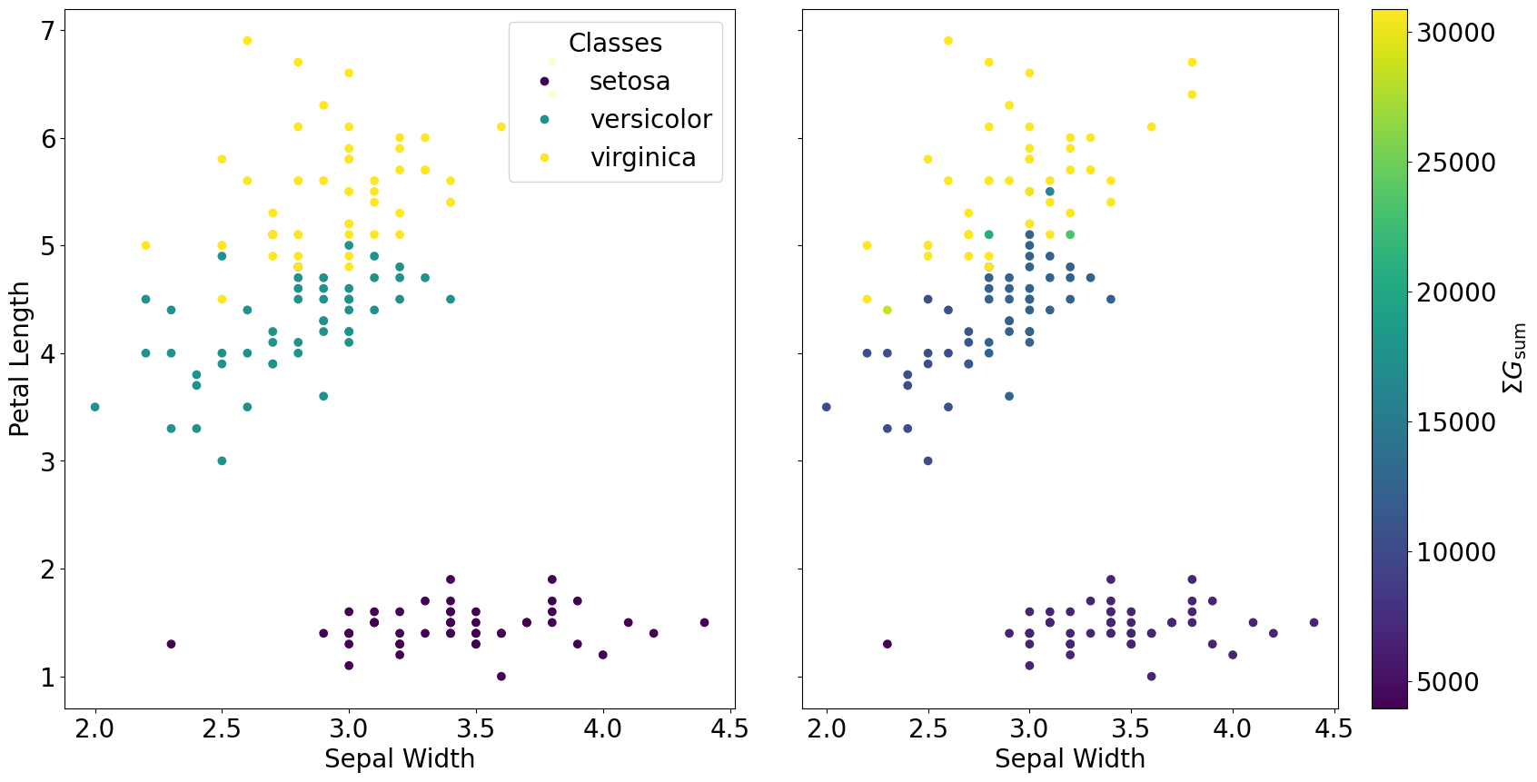
In the simplest case, add all gsum values together to obtain final SCE clustering result

sce_sum = np.zeros((len(iris_data_transformed)))
for i in range(len(ranked_gsum_list)):
    current_cluster_mask = np.load(f"{file_path}/mask-{map_list[i][2]}-id{map_list[i][1]}.npy")
    sce_sum += current_cluster_mask

fig, axs = plt.subplots(1, 2, figsize=(20, 10), sharey=True)
fig.subplots_adjust(wspace=0.1)
scatter_ground = axs[0].scatter(iris.data[:,1], iris.data[:,2], c=iris.target, cmap='viridis')
axs[0].set_xlabel('Sepal Width')
axs[0].set_ylabel('Petal Length')
axs[0].legend(scatter_ground.legend_elements()[0], iris.target_names, loc="upper right", title="Classes")
scatter_sce = axs[1].scatter(iris.data[:,1], iris.data[:,2], c=sce_sum, cmap='viridis')
axs[1].set_xlabel('Sepal Width')
cbar = plt.colorbar(scatter_sce, ax=axs[1])
cbar.set_label(r'$\Sigma G_{\rm sum}$')
plt.show()

Visualize the distribution of the SCE values

plt.rcParams.update({'font.size': 14})
plt.figure(dpi=200)
plt.hist(sce_sum, bins=20, color='r', label='SCE Cluster Sum', histtype='step', linewidth=2)
plt.xlabel('SCE Cluster Sum')
plt.ylabel('Frequency')
plt.show()

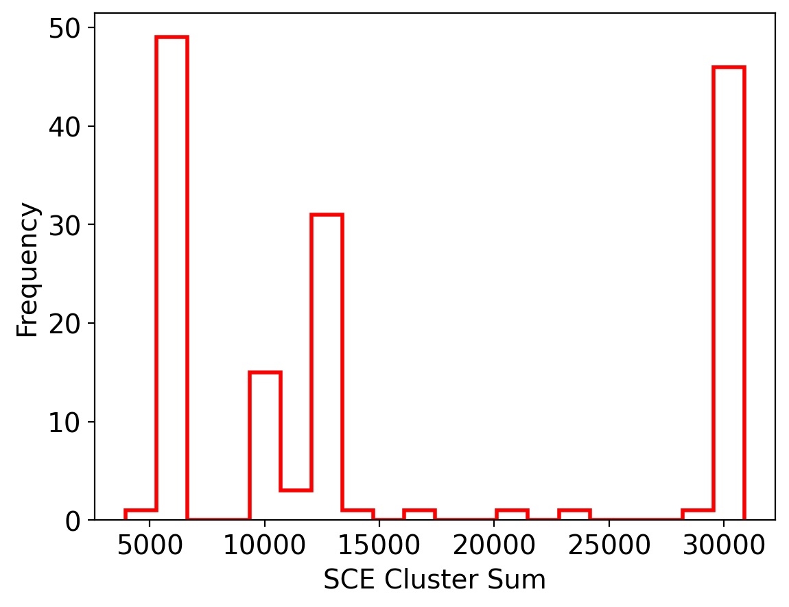
Set signal cutoffs where the data is clustered

signal_cutoff = [8000, 15000]

sce_clusters = np.zeros((len(iris_data_transformed)), dtype=int)
for i in range(len(sce_sum)):
    if sce_sum[i] < signal_cutoff[0]:
        sce_clusters[i] = 0
    elif sce_sum[i] < signal_cutoff[1]:
        sce_clusters[i] = 1
    else:
        sce_clusters[i] = 2

plt.rcParams.update({'font.size': 20})
fig, axs = plt.subplots(1, 2, figsize=(22, 10), sharey=True)
fig.subplots_adjust(wspace=0.1)
scatter_ground = axs[0].scatter(iris.data[:,1], iris.data[:,2], c=iris.target, cmap='viridis')
axs[0].set_xlabel('Sepal Width')
axs[0].set_ylabel('Petal Length')
axs[0].legend(scatter_ground.legend_elements()[0], iris.target_names, loc="upper right", title="Classes")
scatter_sce = axs[1].scatter(iris.data[:,1], iris.data[:,2], c=sce_clusters, cmap='viridis')
axs[1].set_xlabel('Sepal Width')
axs[1].legend(scatter_sce.legend_elements()[0], np.unique(sce_clusters), loc="upper right", title="SCE")
plt.show()

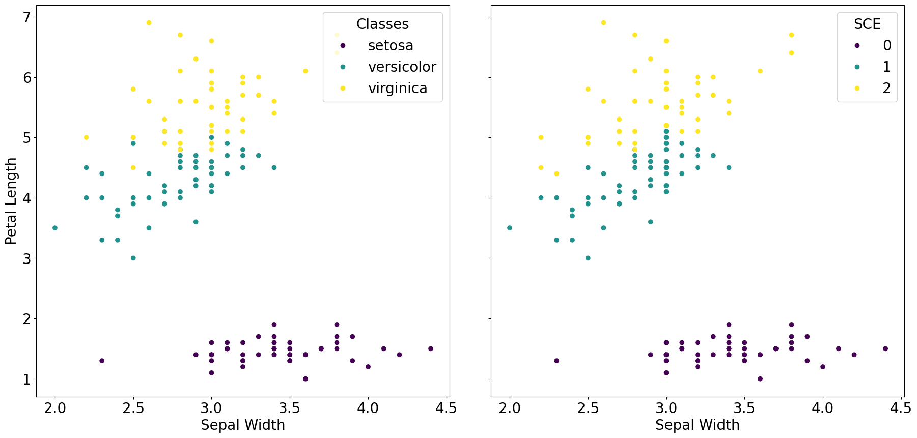
Compare real labels to SCE clustering

# Assign cluster number to class label; change manually
label_map = {'setosa' : 0, 'versicolor' : 1, 'virginica' : 2}
correct_label = 0

for i in range(len(sce_clusters)):
    if int(sce_clusters[i]) == label_map[iris.target_names[iris.target[i]]]:
        correct_label += 1

print("Number of correct predictions: ", correct_label)
print("Accuracy = ", correct_label/len(sce_clusters) * 100, "%")

# Precision and Recall by class
precision = np.zeros(3)
recall = np.zeros(3)

for i in range(3):
    tp = 0
    fp = 0
    fn = 0
    for j in range(len(sce_clusters)):
        if int(sce_clusters[j]) == label_map[iris.target_names[i]]:
            if iris.target[j] == i:
                tp += 1
            else:
                fp += 1
        else:
            if iris.target[j] == i:
                fn += 1
    precision[i] = tp/(tp+fp)
    recall[i] = tp/(tp+fn)

print("Precision: ", [float(np.round(precision[i],4))*100 for i in range(3)], "%")
print("Recall: ", [float(np.round(recall[i],4))*100 for i in range(3)], "%")

Number of correct predictions:  142
Accuracy =  94.66666666666667 %
Precision:  [100.0, 92.0, 92.0] %
Recall:  [100.0, 92.0, 92.0] %